In the early 1970s, plate tectonics was still a young and contested theory. One of its most stubborn puzzles was the opening of the South Atlantic Ocean. Geologists had two competing models: symmetric spreading, where new crust forms equally on both sides of a mid-ocean ridge, and asymmetric spreading, where one side grows faster. Without direct seafloor samples or precise age dates, the debate simmered for years. The resolution came from an unexpected source: the oxygen isotope ratios in the shells of tiny marine organisms called foraminifera.

A Plate Tectonics Riddle That Divided Geologists

The South Atlantic is a textbook example of continental drift: the coastlines of South America and Africa fit together like puzzle pieces. But the details of how they separated remained unclear. The magnetic stripes on the seafloor, which record reversals of Earth's magnetic field, provided a rough chronology, but the ages of the oldest stripes near the continental margins were poorly constrained. Two camps emerged. One argued that spreading was symmetric, with the ridge axis remaining stationary relative to the mantle. The other proposed asymmetric spreading, where the ridge migrated, causing one flank to spread faster.

The dispute mattered beyond academic curiosity. Symmetric spreading implied a simple, uniform process, while asymmetric spreading suggested more complex mantle dynamics. Resolving it required accurate ages for the magnetic anomalies on both sides of the ridge. But the standard tool—biostratigraphy using fossil assemblages—only gave resolution to within a few million years, too coarse to distinguish between models that predicted differences of just a few millimeters per year in spreading rate.

By the late 1970s, the debate had reached an impasse. Each camp could cite magnetic anomaly patterns that seemed to support their view, but the age control was too weak to rule out either model. The South Atlantic became a test case for whether plate tectonics operated as a steady, symmetric machine or a more erratic process.

What the field needed was a global time scale accurate to within a few hundred thousand years—something that could tie together magnetic anomalies, sediment cores, and tectonic events across the ocean basin. That time scale would come from an unlikely source: the deep-sea sediment cores collected by paleoclimatologists.

Why Foraminifera Shells Record Ocean Chemistry

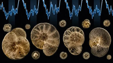
Foraminifera are single-celled marine organisms that build tiny shells, or tests, from calcium carbonate. As they grow, they incorporate oxygen atoms from seawater into their shells. The ratio of the stable isotopes oxygen-18 to oxygen-16—written as δ18O—depends on two main factors: the temperature of the water and the global ice volume. When ice sheets grow, they preferentially lock up light oxygen-16, leaving seawater enriched in oxygen-18. Foraminifera shells preserve this signal.

When foraminifera die, their shells sink to the seafloor and accumulate in sediment layers. By drilling long sediment cores and measuring δ18O in foraminifera shells at different depths, scientists can reconstruct a record of past climate. The deeper the sample, the older the climate. This downcore isotope curve becomes a continuous archive of glacial-interglacial cycles.

The beauty of the method is that it works globally. Foraminifera live in oceans worldwide, and their δ18O signals are broadly synchronous because ice volume changes affect all ocean basins. A peak in δ18O corresponds to a glacial maximum, a trough to an interglacial. These peaks and troughs form a pattern that can be correlated from core to core, creating a global stratigraphic framework.

But raw δ18O curves are not clocks. They show relative changes, not absolute ages. To turn them into a time scale, scientists needed a way to assign numerical ages to the pattern. That breakthrough came from orbital tuning.

The Shackleton Curve That Became a Global Ruler

In the 1970s, Nick Shackleton, a paleoclimatologist at the University of Cambridge, pioneered the use of oxygen isotopes from deep-sea cores to study ice ages. Working with cores from the Pacific Ocean, he produced a δ18O record that extended back hundreds of thousands of years. The curve showed a clear, repeating pattern of glacial-interglacial cycles. Shackleton and his colleagues numbered these cycles—Marine Isotope Stages (MIS)—starting with MIS 1 for the present interglacial and counting backward.

The key insight was that these cycles matched the predictions of Milutin Milankovitch's theory, which linked ice ages to variations in Earth's orbit: eccentricity (roughly 100,000-year cycles), obliquity (roughly 41,000-year cycles), and precession (roughly 23,000-year cycles). By tuning the δ18O curve to orbital parameters, scientists could assign precise ages to each stage. This orbital tuning gave the curve a resolution of a few thousand years—far better than biostratigraphy.

Shackleton's curve became the gold standard for Quaternary chronology. Paleoclimatologists used it to date ice cores, loess deposits, and coral terraces. But its utility extended far beyond climate science. The same curve could be used to date any marine sediment core that contained foraminifera, regardless of location. It provided a global time scale that could be applied to tectonic questions.

By the early 1980s, the Shackleton curve had been extended to cover the past roughly 2.5 million years. For the South Atlantic, which opened roughly 100 million years ago, this was far too young. But the method—orbital tuning of δ18O—could be applied to older sediments, using the same principles. The challenge was finding cores old enough to capture the early opening history.

One notable extension came from the work of James Zachos and colleagues, who compiled a global δ18O stack for the entire Cenozoic, covering the past roughly 65 million years. This stack, built from thousands of measurements across dozens of Deep Sea Drilling Project (DSDP) and Ocean Drilling Program (ODP) cores, provided a continuous record of climate change that could be used to date sediments from the early South Atlantic. The stack was tuned to orbital cycles for the younger portion and to a combination of magnetostratigraphy and cyclostratigraphy for the older part. Although the uncertainties grew for older sediments—typically in the range of tens to hundreds of thousands of years—the stack still offered far better resolution than biostratigraphy alone.

Bridging Oceans: How an Isotope Record Reached Tectonics

The South Atlantic margins are flanked by thick sediment piles, deposited as the ocean widened. These sediments contain foraminifera, but their δ18O records are complicated by local temperature changes and diagenesis. Still, the global pattern of ice volume changes is preserved, and the orbital tuning approach could be applied to Cenozoic sediments. The key was to use multiple cores and correlate them to the global δ18O stack.

In the late 1970s, the Deep Sea Drilling Project (DSDP) had recovered several cores from the South Atlantic. These cores contained magnetic reversal records and foraminifera. By measuring δ18O in the same cores, scientists could link the magnetic chrons—numbered intervals of normal or reversed polarity—to the global isotope curve. This gave each magnetic chron a precise age, rather than the rough estimates from biostratigraphy.

The critical step was to date the oldest magnetic anomalies on each side of the ridge. If spreading was symmetric, the oldest anomalies should be the same age on both flanks. If asymmetric, one flank should show older anomalies. The δ18O curve provided the ages needed to test this.

The work was painstaking. Each core had to be sampled at high resolution, the foraminifera picked and cleaned, and the isotope ratios measured on a mass spectrometer. The resulting δ18O curves were then correlated to the global stack, and the ages of magnetic reversals were interpolated. The uncertainties were still several hundred thousand years, but that was enough to distinguish between spreading models that predicted age differences of millions of years.

A key example came from DSDP Site 522, located on the African flank of the Mid-Atlantic Ridge. There, the sediment core preserved a continuous record of magnetic reversals and foraminifera shells. By measuring δ18O in the same core, researchers could assign ages to the reversals with an uncertainty of roughly plus or minus 200,000 years. This allowed them to calculate the spreading rate on that flank. A similar analysis on the South American flank, using DSDP Site 519, gave a nearly identical rate. The two rates agreed within roughly 0.5 millimeters per year—well within the error bars.

Symmetric Spreading Confirmed by Oxygen Isotopes

The definitive study came in 1982, when geophysicist Steven Cande and paleoceanographer John Mutter published a paper in the Journal of Geophysical Research. They used δ18O-based ages from DSDP cores to date magnetic anomalies on both sides of the Mid-Atlantic Ridge in the South Atlantic. Their results were clear: the ages of corresponding anomalies matched within the uncertainties, typically less than one million years. The spreading rates on the two flanks agreed to within about one millimeter per year.

This ruled out the asymmetric spreading model for the South Atlantic. The ridge had remained essentially stationary relative to the mantle since the opening began, and crust had been added equally on both sides. The symmetric model was confirmed. The oxygen isotope curve had settled a decade-long debate.

The impact was immediate. Other ocean basins were reexamined using the same approach. The Indian Ocean, the North Atlantic, and the Pacific all showed symmetric spreading within the resolution of the method. The asymmetric model, which had been a serious contender, was relegated to rare, localized exceptions—usually near subduction zones or hot spots.

But the study also highlighted the power of cross-disciplinary borrowing. A tool developed for climate science—the orbital-tuned δ18O curve—had solved a tectonic problem. It was not a grand theory but a calibration device, a ruler that could be applied across fields. The success inspired other collaborations between paleoclimatologists and geophysicists, leading to improved time scales for the entire Cenozoic.

Methodological Lessons for Cross-Disciplinary Science

The story of the oxygen isotope curve and the South Atlantic offers several lessons for how scientific tools move between fields. First, the isotope curve was not a tectonic theory; it was a measurement standard. Its precision came from orbital tuning, which was independent of the tectonic processes being studied. This independence gave it credibility among geophysicists who might have been skeptical of a climate-derived chronology.

Second, the collaboration required both sides to understand each other's uncertainties. Paleoclimatologists had to explain the assumptions behind orbital tuning—that sedimentation rates are roughly constant between tie points, that the δ18O signal is globally synchronous, and that diagenesis has not altered the shells. Geophysicists had to accept that the ages were not absolute but probabilistic, with error bars that could be quantified.

p>Third, the success depended on a shared reference frame. The numbered marine isotope stages provided a common language that allowed researchers in different fields to compare data. A magnetic anomaly in the South Atlantic could be assigned to MIS 8 or MIS 10, and anyone familiar with the isotope curve knew its approximate age. This shared vocabulary was essential for the cross-disciplinary dialogue.

Finally, the episode showed the value of open data. Shackleton's original δ18O curves were published and made available to the community. Other researchers could replicate his measurements, extend them to new cores, and test his correlations. This transparency built trust and allowed the curve to become a community standard, much like the standard reference materials used in analytical chemistry.

What the Curve Still Cannot Tell Us

For all its power, the oxygen isotope approach has limitations. The most fundamental is the assumption of constant sedimentation rate between tie points. If sedimentation is episodic—due to turbidity currents, winnowing, or dissolution—the ages derived from linear interpolation can be off by hundreds of thousands of years. This is a particular problem in tectonically active basins, where slumping and erosion are common.

Another issue is that the δ18O signal is not purely global. Local temperature changes, salinity variations, and vital effects (biological fractionation by different foraminifera species) can introduce noise. While stacking many cores reduces this noise, it never disappears. The global stack is an average, and individual cores may deviate from it by several tenths of a per mil, corresponding to age uncertainties of tens of thousands of years.

p>For the South Atlantic case, these uncertainties were acceptable because the age differences between symmetric and asymmetric models were large. But for finer-scale tectonic questions—such as whether spreading rates vary on million-year timescales—the isotope curve may not be precise enough. Modern geochronology offers alternatives: argon-argon dating of volcanic ash layers, uranium-lead dating of zircons, and magnetostratigraphy combined with cyclostratigraphy. These methods can achieve precisions of a few thousand years, but they require suitable materials that are not always present in deep-sea cores.

p>Despite these caveats, the oxygen isotope curve remains a powerful tool. It has been extended back to the Cretaceous using bulk carbonate and other proxies, and it continues to be refined with new cores and higher-resolution measurements. The lesson of the South Atlantic is that even an imperfect ruler, if it is consistent and widely accepted, can resolve debates that seemed intractable. The foraminifera shells that built that ruler are still accumulating on the seafloor, adding new pages to the archive of Earth history.

p>One notable counter-argument came from researchers who pointed out that the δ18O curve, while excellent for correlating events, might not capture short-lived tectonic pulses. For instance, if the spreading rate changed abruptly over a few hundred thousand years, the isotope curve's resolution of roughly 20,000 to 30,000 years might still miss it. However, for the South Atlantic debate, the question was about the long-term average spreading rate over millions of years, not short-term fluctuations. The isotope curve was well suited to that question.

p>Another trade-off involves the choice of foraminifera species. Different species live at different depths in the water column and exhibit different vital effects. Benthic foraminifera, which live on the seafloor, record deep-water conditions and are less affected by surface temperature changes. Planktic foraminifera, which live near the surface, record mixed-layer conditions. For the South Atlantic study, researchers typically used benthic species because their δ18O signal is more directly tied to global ice volume, but they had to account for the fact that deep-water temperatures also change over glacial-interglacial cycles. This introduced an additional uncertainty of roughly plus or minus 0.2 per mil, corresponding to an age uncertainty of roughly plus or minus 10,000 to 20,000 years. Despite these complications, the overall pattern remained robust.