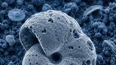
Foraminifera—tiny, shelled protists that drift through the world's oceans—are the workhorses of paleoclimatology. Their calcium carbonate shells, preserved in seafloor sediments, carry chemical signatures that scientists use to reconstruct past ocean temperatures, ice volumes, and carbon cycles. But those shells do not all survive the journey from surface waters to the sediment archive. A quiet, selective process called dissolution—the gradual etching and thinning of carbonate in corrosive deep waters—removes some species before they ever become fossils. That removal is not random. It preferentially targets thin-shelled species, and it biases the very signals that underpin global temperature stacks.

The effect is subtle enough to escape notice in individual cores, but when hundreds of records are stacked to produce a global picture, the bias can accumulate. Some estimates place the distortion at roughly 0.3–0.5°C in reconstructed sea surface temperatures (SST)—a non-trivial fraction of the 1–2°C shifts that define glacial-interglacial cycles. This is not a story of catastrophic error, but of methodological drift: a systematic skew that, if unaccounted for, can bend the shape of Earth's climate history.

This article walks through how dissolution bias works, where it hides in the data, and what the paleoclimate community is doing about it. It is a focused explainer with named studies and concrete numbers, written for readers who want to see behind the curtain of how paleoclimate evidence is actually produced.

The Unseen Filter in Paleoclimate Archives

Deep-sea sediments accumulate slowly—typically a few centimeters per thousand years. Foraminifera shells, which rain down from the sunlit surface layer, make up a large fraction of that carbonate mud. In many regions, these shells are the primary material for geochemical analyses: oxygen isotope ratios (δ¹⁸O) record ice volume and temperature, while magnesium-to-calcium ratios (Mg/Ca) serve as a thermometer for past seawater temperature.

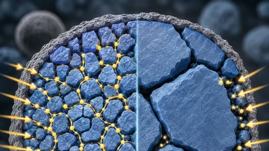
But the ocean is not a neutral storage medium. Below a certain depth—the lysocline—seawater becomes undersaturated with respect to calcite, the mineral form of foraminifera shells. Dissolution begins. The process is not uniform: thin-shelled species, which have a higher surface-area-to-volume ratio, dissolve faster than thick-shelled ones. Over time, the sediment assemblage becomes enriched in robust, dissolution-resistant taxa. This selective loss is the filter through which all deep-sea carbonate records must pass.

The bias is not limited to species counts. Shell chemistry also changes during dissolution. Magnesium, which substitutes for calcium in the crystal lattice, is preferentially removed because Mg–O bonds are weaker than Ca–O bonds. As a result, partially dissolved shells yield lower Mg/Ca ratios than their pristine counterparts, mimicking a cooler temperature signal. Similarly, oxygen isotopes can shift if dissolution preferentially removes isotopically heavy or light domains within the shell, though the direction and magnitude depend on the specific species and dissolution intensity.

These effects are well documented in laboratory experiments and in core-top calibrations. Yet many global compilations—the stacks that define the timing and amplitude of past climate events—are built from records that do not explicitly correct for dissolution. The assumption is that dissolution is either negligible or randomly distributed, but that assumption may be wrong.

How Dissolution Skews Mg/Ca Thermometry

The Mg/Ca paleothermometer is one of the most widely used tools in paleoceanography. The ratio of magnesium to calcium in foraminifera shells increases exponentially with temperature, with a sensitivity of roughly 8–10% per °C. A measurement precision of 0.1°C is possible in ideal conditions. But dissolution degrades that precision.

In a 2014 study, scientists compared Mg/Ca values from well-preserved and artificially dissolved shells of the planktonic species Globigerinoides ruber. They found that dissolution could reduce Mg/Ca by 15–25%, equivalent to an apparent cooling of 1.5–2.5°C. This is a worst-case scenario—laboratory dissolution is aggressive—but it illustrates the potential magnitude. In natural sediments, the effect is smaller but still detectable: core-top studies show that Mg/Ca decreases with increasing water depth, even when surface temperature is constant, because dissolution intensifies with pressure and carbonate undersaturation.

Regional stacks that combine records from different depths inadvertently mix dissolution states. A core from 3,000 meters may yield systematically lower Mg/Ca than a core from 2,000 meters, even if both record the same past temperature. When these records are averaged into a global stack, the depth-dependent bias can produce artificial trends. For the last glacial maximum, some stacks show a cooling of roughly 2–3°C in the tropics, but a portion of that signal may reflect dissolution, not actual ocean change.

Efforts to correct for dissolution typically use a depth-correction formula derived from core-top calibrations. One common approach applies a linear correction of about 0.1°C per 500 meters below the lysocline. But this is a blunt instrument. The actual sensitivity varies with species, sedimentation rate, and bottom-water chemistry. Overcorrecting could introduce its own bias, smoothing out real spatial variability in past ocean conditions.

Oxygen Isotopes and the Dissolution Imprint

Oxygen isotope ratios (δ¹⁸O) in foraminifera shells are a dual proxy: they reflect both temperature and the isotopic composition of seawater, which itself tracks ice volume. Dissolution complicates this signal because it can alter the shell's internal isotopic heterogeneity.

Foraminifera build their shells in layers, with different layers deposited at different times of day or under different physiological states. The outermost layers, which are more porous and less dense, tend to dissolve first. These layers also tend to have slightly different δ¹⁸O values than the inner layers—sometimes heavier, sometimes lighter, depending on the species and the growth environment. When dissolution strips away these outer layers, the remaining shell material records a biased average.

A 2018 study examined this effect in the benthic species Cibicidoides wuellerstorfi, a staple of deep-sea isotope records. The authors found that partial dissolution could shift δ¹⁸O by 0.1–0.3‰—a small but systematic offset. In the context of glacial-interglacial cycles, where the total δ¹⁸O change is about 1.5–2‰, a 0.2‰ bias translates to roughly 10–15% of the signal. This is enough to shift the timing of inferred ice-volume changes by a few thousand years, depending on the sedimentation rate.

Stacked records that average many cores partially cancel random noise, but they do not cancel systematic biases. If cores from shallower depths (less dissolution) are preferentially included in one time interval and deeper cores in another, the stack can develop a spurious trend. This is particularly relevant for the last deglaciation, when sea level rose and the carbonate compensation depth (CCD) may have shifted, altering the dissolution regime across ocean basins.

Some researchers advocate for using only the inner, more resistant portion of the shell for isotopic analysis, a technique called "carapace" or "inner layer" analysis. This reduces the dissolution bias but requires additional sample preparation and may not be feasible for all cores. The trade-off is between sample throughput and data quality—a familiar tension in paleoclimate science.

Stacking Records: When Regional Distortions Become Global

Global stacks are powerful tools. They combine dozens or hundreds of individual records to produce a single curve that represents Earth's average climate history. The most famous example is the LR04 benthic δ¹⁸O stack, which spans 5.3 million years and is used as a template for correlating marine and terrestrial records. These stacks are built on the assumption that regional biases average out. But dissolution bias is not random—it is correlated with water depth, which itself varies systematically across ocean basins.

The Pacific Ocean, for example, has a deeper lysocline than the Atlantic because Pacific deep waters are older and more corrosive. A stack that includes more Pacific cores from shallower depths may appear to show different glacial-interglacial amplitudes than a stack dominated by Atlantic cores. When these stacks are combined into a global mean, the depth-correlated bias can produce artifacts that resemble genuine climate variability.

A 2020 study tested this by simulating dissolution bias in a synthetic stack. The authors applied a depth-dependent correction to Mg/Ca records from 50 cores and found that the uncorrected stack overestimated glacial cooling by about 0.4°C on average, with larger errors in the tropics. The correction reduced the mismatch between proxy-based reconstructions and climate model simulations, suggesting that some of the previously noted proxy-model discrepancy may stem from dissolution bias.

But correction methods are not yet standardized. Some labs use a simple depth threshold, excluding cores below 3,500 meters. Others apply a species-specific correction based on the ratio of dissolution-resistant to dissolution-prone taxa. Still others rely on a physical model of pore-water chemistry to estimate in situ dissolution rates. Each approach has different assumptions and uncertainties, and the choice of correction can alter the shape of the stack.

The community is moving toward more transparent reporting: many journals now require authors to state the dissolution state of their samples and to describe any correction applied. But legacy stacks, built from decades of published data, may not have this information. Revisiting and correcting those stacks is a painstaking task that requires reanalyzing original sediment samples or applying approximate corrections based on core metadata. It is work that is underway, but far from complete.

Correcting the Record Without Overcorrecting

There is a fine line between correcting a bias and introducing a new one. Overzealous correction can remove real signals—for instance, a genuine cooling trend that happens to correlate with water depth because ocean circulation changed. The challenge is to distinguish between dissolution artifacts and true climate variability.

One promising approach is to use independent proxies that are less sensitive to dissolution. For example, the clumped isotope thermometer (Δ₄₇) measures the abundance of ¹³C–¹⁸O bonds in carbonate, which is thermodynamically controlled and less affected by selective dissolution than Mg/Ca. Clumped isotope analyses require larger sample sizes and more precise mass spectrometry, but they offer a way to validate Mg/Ca-based temperature estimates in dissolution-prone settings.

Another strategy is to quantify dissolution directly using the ratio of calcite to aragonite or the fragmentation index of foraminifera shells. Cores with high fragmentation likely experienced significant dissolution, and their geochemical data can be downweighted or excluded from stacks. This approach has been used in several regional compilations, but it is not yet standard practice globally.

Statistical methods also help. Bayesian hierarchical models can incorporate dissolution as a latent variable, estimating its effect alongside the climate signal. These models require careful prior specification and are computationally intensive, but they provide a principled way to propagate uncertainty. A 2022 study used such a model to reanalyze the Mg/Ca-based temperature stack for the last 800,000 years and found that dissolution bias accounted for roughly 0.2–0.3°C of the apparent glacial-interglacial amplitude.

None of these corrections is perfect. The paleoclimate community is still debating the magnitude and spatial pattern of dissolution bias. Reasonable people disagree on whether the effect is large enough to warrant retrospective correction of all published stacks. Some argue that the bias is small relative to other uncertainties, such as the calibration of the Mg/Ca thermometer itself. Others contend that even a 0.3°C bias matters when the goal is to constrain climate sensitivity—the amount of warming per doubling of CO₂—to within 1°C.

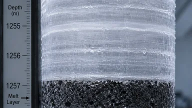
The debate is healthy. It reflects a maturing field that is learning to account for the messy realities of the sediment archive. Similar methodological self-examination has reshaped other areas of paleoclimate science, such as the correction for ice-core melt layers that can resequence a Greenland temperature stack, as discussed in a related article on this site. The key is to keep the conversation empirical, grounded in concrete measurements and testable hypotheses.

What This Means for Climate Sensitivity Estimates

Climate sensitivity—the equilibrium global warming from a doubling of atmospheric CO₂—is one of the most important numbers in climate science. Paleoclimate estimates of sensitivity often rely on SST reconstructions from foraminifera Mg/Ca and δ¹⁸O. If those reconstructions are biased by dissolution, the inferred sensitivity could be off by a measurable amount.

For the last glacial maximum, roughly 21,000 years ago, CO₂ was about 190 ppm, compared to preindustrial 280 ppm. The radiative forcing difference is about 3.7 W/m². Reconstructed global cooling ranges from 4–7°C. The resulting climate sensitivity estimate depends on the exact temperature change. A 0.5°C bias in SST—from dissolution or any other source—translates to roughly a 0.3°C shift in estimated equilibrium sensitivity, assuming a linear relationship. That is not negligible when the uncertainty range for sensitivity is often cited as 1.5–4.5°C.

Moreover, dissolution bias may affect different time intervals differently. If glacial sediments experienced more dissolution than interglacial sediments—because of changes in ocean circulation or the CCD—the amplitude of glacial-interglacial temperature change could be systematically distorted. This would affect not only sensitivity estimates but also the timing of ice-sheet growth and decay.

A 2019 study compared SST reconstructions from the last glacial maximum using two different proxies: Mg/Ca and the alkenone unsaturation index (U³⁷′), which is derived from organic compounds produced by haptophyte algae. Alkenones are not affected by carbonate dissolution. The study found that Mg/Ca-based SSTs were on average 0.4°C cooler than alkenone-based SSTs in the tropics, consistent with a dissolution bias. However, the two proxies also differ in their seasonal and depth habitats, so the discrepancy cannot be attributed solely to dissolution.

Resolving these ambiguities requires more direct measurements of dissolution in sediment cores. X-ray microtomography can now image the internal structure of foraminifera shells at micron resolution, revealing the degree of etching and thinning. This technique is still too slow for routine use, but it provides a ground truth for calibrating faster, bulk-chemical methods. As these tools become more accessible, the paleoclimate community will be better equipped to account for dissolution bias in a rigorous, site-specific way.

In the meantime, the message for non-specialists is simple: paleoclimate records are not raw data. They are the product of a long chain of processes—biological, chemical, and physical—that shape what is preserved in the sediment. Dissolution is one link in that chain, and it deserves attention. The stacks that define our understanding of Earth's climate history are only as strong as their weakest correction.

For readers interested in parallel methodological challenges, see the article on how an unreported cathode annealing ramp rate skewed a battery lifetime competition, which highlights similar issues of hidden experimental bias in materials science.